Mathematics
Mathematics
Welcome to my Mathematics page — where I document topics I teach and explore, from basic rules to worked examples.
Using Your Calculator to Find Basic Angles
Inverse Trigonometric Functions
This video explains inverse trigonometric functions — arcsin, arccos, and arctan — and how they differ from regular trig functions like sin, cos, and tan.
Function vs. Inverse Function
A function $f$ takes an input and gives one output: $f(x) = y$. An inverse function $f^{-1}$ reverses that — it takes the output and gives back the original input: $f^{-1}(y) = x$.
Key idea: if $f$ and $f^{-1}$ undo each other, then $f^{-1}(f(x)) = x$.
Important condition: a function only has an inverse if it’s one-to-one (each output comes from exactly one input). This matters a lot for trig functions, since $\sin(x)$, $\cos(x)$, $\tan(x)$ repeat their values over and over — so we have to restrict their domain before we can invert them.
Notation
- $f^{-1}(x)$ means “the inverse function of $f$” — not $\frac{1}{f(x)}$
- Same for trig: $\sin^{-1}(x) \neq \frac{1}{\sin(x)}$. That’s why many textbooks prefer arcsin, arccos, arctan — it avoids the confusion entirely
Arcsine, Arccosine, Arctangent
| Function | Restricted domain of original | Range of inverse |
|---|---|---|
| $\arcsin(x) = \sin^{-1}(x)$ | $\sin(x)$ restricted to $[-\frac{\pi}{2}, \frac{\pi}{2}]$ | $[-\frac{\pi}{2}, \frac{\pi}{2}]$ |
| $\arccos(x) = \cos^{-1}(x)$ | $\cos(x)$ restricted to $[0, \pi]$ | $[0, \pi]$ |
| $\arctan(x) = \tan^{-1}(x)$ | $\tan(x)$ restricted to $(-\frac{\pi}{2}, \frac{\pi}{2})$ | $(-\frac{\pi}{2}, \frac{\pi}{2})$ |
In plain terms: $\arcsin(x)$ answers the question “what angle has a sine of $x$?” — same logic for the other two.
Example: $\sin(30°) = 0.5$, so $\arcsin(0.5) = 30°$.
Basic Differentiation Rule
This video walks through the basic differentiation rule, $\frac{d}{dx}(x^{n}) = nx^{n-1}$, and how it applies to polynomial functions.
Summary & Examples
- Derivative of $y=f(x)$ with respect to $x$ is denoted by $\frac{dy}{dx}, \frac{df}{dx}, f^{\prime}(x)$.
Power Rule
(a) $f(x)=x^{6}$
(b) $g(q)=\sqrt{q}$
(c) $h(p)=\frac{1}{p^{2}}$
Solution:
(a) \(\frac{df}{dx}=6x^{5}\)
(b) \(g(q)=\sqrt{q}=q^{1/2} \Rightarrow g^{\prime}(q)=\frac{1}{2}q^{-1/2}\)
(c) \(h(p)=\frac{1}{p^{2}}=p^{-2} \Rightarrow h^{\prime}=-2p^{-3}\)
Constant Multiple Rule
(a) $h(x)=5x^{3}$
(b) $g(x)=2\ln x$
Basic Differentiation - Product Rule
An introduction to the Product Rule in differentiation — how to find the derivative of a function that is the product of two other functions.
Worked Example
Find the derivative of $f(x)=x^{2}\sin(x)$.
Solution:
The product rule states that for two differentiable functions $u(x)$ and $v(x)$:
\[\frac{d}{dx}[u(x)\cdot v(x)]=u^{\prime}(x)v(x)+u(x)v^{\prime}(x)\]Step 1 : Identify the components:
- $u(x)=x^{2} \Longrightarrow u^{\prime}(x)=2x$
- $v(x)=\sin(x) \Longrightarrow v^{\prime}(x)=\cos(x)$
Step 2 : Apply the product rule:
\[f^{\prime}(x)=(2x)\sin(x)+x^{2}\cos(x)\]Step 3 : Simplify (optional):
\[f^{\prime}(x)=x(2\sin(x)+x\cos(x))\]Basic Differentiation - Quotient Rule
The Quotient Rule tells you how to differentiate a function that is one function divided by another.
Formula
\[\frac{d}{dx}\left[\frac{u(x)}{v(x)}\right] = \frac{u'(x)\,v(x) - u(x)\,v'(x)}{[v(x)]^2}\]A common way to remember it: “low d-high minus high d-low, over the square of what’s below” — where “high” = $u$ (numerator) and “low” = $v$ (denominator).
How to Apply It
Step 1 — Identify the components: Split the function into $u(x)$ (top) and $v(x)$ (bottom), then find $u’(x)$ and $v’(x)$ separately.
Step 2 — Plug into the formula: \(f'(x) = \frac{u'v - uv'}{v^2}\)
Step 3 — Simplify (combine like terms in the numerator, factor if possible).
Worked Example
Find the derivative of $f(x) = \dfrac{\sin(x)}{x}$.
- $u(x) = \sin(x) \Rightarrow u’(x) = \cos(x)$
- $v(x) = x \Rightarrow v’(x) = 1$
Common mistake to watch for: the order in the numerator matters — it’s $u’v - uv’$, not $uv’ - u’v$. Swapping the order flips the sign of the whole answer.
Integration of Fundamental Functions
Integration is the reverse of differentiation. For each standard function, remember its antiderivative plus a constant $C$ (since the derivative of any constant is 0).
Standard Functions
| $f(x)$ | $\int f(x)\,dx$ |
|---|---|
| $x^k$ | $\dfrac{x^{k+1}}{k+1} + C$ (Power Rule, $k \neq -1$) |
| $e^x$ | $e^x + C$ |
| $\dfrac{1}{x}$ | $\ln\lvert x \rvert + C$ |
| $\sin x$ | $-\cos x + C$ |
| $\cos x$ | $\sin x + C$ |
Key points to note:
-
$x^k$ rule breaks when $k = -1$ (that’s exactly when $1/x$ takes over, giving $\ln x $ instead) - $e^x$ is unique — it integrates to itself
- Sign flips for $\sin x$: integrating gives $-\cos x$, not $+\cos x$ (easy to mix up)
- Always add $+C$ — dropping it is the most common mistake
Example: $\int t^3\, dt = \dfrac{t^4}{4} + C$
When a Function Doesn’t Match a Standard Form
If the integral isn’t directly one of these standard results, a technique is needed to reduce it to one. Three common methods (not an exhaustive list):
- Integration by Substitution — rewrite the integral in terms of a new variable to simplify it into a standard form
- Integration by Parts — used for a product of two functions
- Partial Fractions — break a complex rational function into simpler fractions, then integrate each term using the standard results above
Integration by Substitution (Recognition Method)
This method works when the integrand contains a function $f(x)$ and its derivative $f’(x)$ together. Once you recognize the pattern, you can integrate directly — no formal substitution needed.
Three Standard Forms
1. \(\int \frac{f'(x)}{f(x)}\,dx = \ln\lvert f(x) \rvert + C\)
Derivation: since $\dfrac{d}{dx}\ln\lvert f \rvert = \dfrac{f’}{f}$, integrating both sides gives the result.
2. \(\int [f(x)]^n f'(x)\,dx = \frac{[f(x)]^{n+1}}{n+1} + C\)
Derivation: let $u = f(x)$, so $du = f’(x)\,dx$. This turns the integral into $\int u^n\,du = \dfrac{u^{n+1}}{n+1} + C$.
3. \(\int e^{f(x)} f'(x)\,dx = e^{f(x)} + C\)
Derivation: since $\dfrac{d}{dx}e^f = e^f \cdot f’$, integrating both sides gives the result.
Worked Example 1 — Recognition Method
\[\int \frac{e^{2x}}{e^{2x}-2}\,dx\]Step 1 — Identify $f(x)$ and $f’(x)$: Let $f(x) = e^{2x} - 2$, so $f’(x) = 2e^{2x}$.
Step 2 — Rewrite the numerator to match $f’(x)$: \(e^{2x} = \frac{1}{2}f'(x)\)
Step 3 — Apply Formula 1: \(\int \frac{e^{2x}}{e^{2x}-2}\,dx = \frac{1}{2}\int \frac{f'(x)}{f(x)}\,dx = \frac{1}{2}\ln\lvert e^{2x}-2 \rvert + C\)
Key point: the constant $\frac{1}{2}$ is pulled out to make the numerator match $f’(x)$ exactly — this adjustment step is the main skill to practice with the recognition method.
Worked Example 2 — Change of Variable
Not every integral fits the recognition shortcut directly. Sometimes it’s clearer to formally substitute a new variable $u$, rewrite the entire integral in terms of $u$ (including $x$ itself), integrate, then substitute back.
\[\int x\sqrt{x+1}\,dx\]Step 1 — Choose the substitution: Let $u = x+1$, so $x = u-1$ and $du = dx$.
Step 2 — Rewrite the whole integral in terms of $u$: \(\int x\sqrt{x+1}\,dx = \int (u-1)\sqrt{u}\,du = \int \left(u^{3/2} - u^{1/2}\right) du\)
Step 3 — Integrate using the Power Rule: \(= \frac{2}{5}u^{5/2} - \frac{2}{3}u^{3/2} + C\)
Step 4 — Substitute back $u = x+1$: \(\int x\sqrt{x+1}\,dx = \frac{2}{5}(x+1)^{5/2} - \frac{2}{3}(x+1)^{3/2} + C\)
Key point: unlike Example 1, here $x$ itself had to be rewritten in terms of $u$ (as $u-1$) before integrating — this is the defining feature of the change-of-variable method, as opposed to just spotting a ready-made $f$ and $f’$ pair.
Integration by Parts
This video explains Integration by Parts — a technique for integrating a product of two functions when standard formulas or substitution don’t directly work.
Formula
\[\int u\,dv = uv - \int v\,du\]Used when integrating a product of two functions that doesn’t fit substitution.
How to Choose u and dv
A common guide is LIATE — pick $u$ in this priority order: Logarithmic, Inverse trig, Algebraic, Trigonometric, Exponential. Whichever type appears first in that list becomes $u$; the rest becomes $dv$.
Worked Example
Find $\int x\,e^x\,dx$.
Step 1 — Choose $u$ and $dv$: By LIATE, $x$ (algebraic) ranks above $e^x$ (exponential), so: \(u = x, \quad dv = e^x\,dx\)
Step 2 — Find $du$ and $v$: \(du = dx, \quad v = e^x\)
Step 3 — Apply the formula: \(\int x\,e^x\,dx = x\,e^x - \int e^x\,dx\)
Step 4 — Integrate what’s left and simplify: \(\int x\,e^x\,dx = x\,e^x - e^x + C\)
Key point: the whole trick is choosing $u$ so that $\int v\,du$ ends up simpler than the original integral — here, differentiating $x$ down to $1$ (via $du$) is what made the leftover integral trivial.
Maclaurin Series (Taylor Series at x = 0)
A beginner’s walkthrough of the Maclaurin series — how to build a polynomial approximation of a function purely from its derivatives at zero.
The Idea
A Maclaurin series rewrites a function as an infinite polynomial, built entirely from the function’s derivatives at $x = 0$.
\[f(x) = f(0) + f'(0)x + \frac{f''(0)}{2!}x^2 + \frac{f'''(0)}{3!}x^3 + \cdots = \sum_{n=0}^{\infty} \frac{f^{(n)}(0)}{n!}x^n\]It’s a special case of the Taylor series, centred at $0$ instead of some general point $a$.
Worked Example: Deriving $e^x$
Take $f(x) = e^x$. Every derivative of $e^x$ is $e^x$, so:
| $n$ | $f^{(n)}(x)$ | $f^{(n)}(0)$ |
|---|---|---|
| 0 | $e^x$ | $1$ |
| 1 | $e^x$ | $1$ |
| 2 | $e^x$ | $1$ |
| 3 | $e^x$ | $1$ |
Substituting into the formula:
\[e^x = 1 + x + \frac{x^2}{2!} + \frac{x^3}{3!} + \frac{x^4}{4!} + \cdots \quad \text{(valid for all } x\text{)}\]Worked Example: Deriving $\sin x$
Take $f(x) = \sin x$. Differentiate repeatedly and evaluate at $x=0$:
| $n$ | $f^{(n)}(x)$ | $f^{(n)}(0)$ |
|---|---|---|
| 0 | $\sin x$ | $0$ |
| 1 | $\cos x$ | $1$ |
| 2 | $-\sin x$ | $0$ |
| 3 | $-\cos x$ | $-1$ |
| 4 | $\sin x$ | $0$ |
| 5 | $\cos x$ | $1$ |
The pattern repeats every 4 derivatives ($\sin \to \cos \to -\sin \to -\cos \to \sin \cdots$), and every even-order term is $0$.
\[\sin x = 0 + 1\cdot x + \frac{0}{2!}x^2 + \frac{-1}{3!}x^3 + \frac{0}{4!}x^4 + \frac{1}{5!}x^5 + \cdots\] \[\sin x = x - \frac{x^3}{3!} + \frac{x^5}{5!} - \frac{x^7}{7!} + \cdots \quad \text{(valid for all } x\text{)}\]Only odd powers survive — a direct consequence of $\sin x$ being an odd function.
Standard Expansions Table
| Function | Series | Valid range |
|---|---|---|
| $e^x$ | $1 + x + \dfrac{x^2}{2!} + \dfrac{x^3}{3!} + \cdots$ | all $x$ |
| $\ln(1+x)$ | $x - \dfrac{x^2}{2} + \dfrac{x^3}{3} - \dfrac{x^4}{4} + \cdots$ | $-1 < x \le 1$ |
| $\ln(1-x)$ | $-x - \dfrac{x^2}{2} - \dfrac{x^3}{3} - \dfrac{x^4}{4} - \cdots$ | $-1 \le x < 1$ |
| $\dfrac{1}{1+x}$ | $1 - x + x^2 - x^3 + \cdots$ | $\lvert x \rvert < 1$ |
| $\dfrac{1}{1-x}$ | $1 + x + x^2 + x^3 + \cdots$ | $\lvert x \rvert < 1$ |
| $\sin x$ | $x - \dfrac{x^3}{3!} + \dfrac{x^5}{5!} - \cdots$ | all $x$ |
| $\cos x$ | $1 - \dfrac{x^2}{2!} + \dfrac{x^4}{4!} - \cdots$ | all $x$ |
Pattern to notice:
- $\sin x$ and $\cos x$ only ever have odd or even powers respectively — because $\sin$ is an odd function and $\cos$ is an even function.
- $\ln(1-x)$ is just $\ln(1+x)$ with every $x \to -x$ — same trick works for $\dfrac{1}{1-x}$ vs $\dfrac{1}{1+x}$.
- $\dfrac{1}{1-x}$ is the geometric series you already know: $1 + x + x^2 + \cdots$
Homogeneous Functions & Euler's Theorem
Definition
A function $f(x, y)$ is homogeneous of degree $n$ if, for every $t$,
\[f(tx,\ ty) = t^n f(x,y)\]Quick test (no need to substitute $t$): add up the powers of $x$ and $y$ in each term. If every term has the same total degree, the function is homogeneous of that degree.
| $f(x,y)$ | Term-by-term degree | Homogeneous? |
|---|---|---|
| $x^2 + 3xy + y^2$ | $2,\ 2,\ 2$ | Yes, degree 2 |
| $x^2y - 2y^3$ | $3,\ 3$ | Yes, degree 3 |
| $\dfrac{x^2+y^2}{xy}$ | numerator deg 2, denominator deg 2 | Yes, degree 0 |
| $x^2 + y$ | $2,\ 1$ | No — mixed degrees |
Euler’s Theorem
If $f(x,y)$ is homogeneous of degree $n$, then
\[x\,f_x + y\,f_y = n\,f(x,y)\]where $f_x = \dfrac{\partial f}{\partial x}$ and $f_y = \dfrac{\partial f}{\partial y}$.
In words: scale each partial derivative by the variable it came from, add them up, and the result is just $n$ times the original function. This gives a quick way to check homogeneity once the derivatives are known, without repeating the $f(tx,ty) = t^n f(x,y)$ substitution.
Worked Example
Question: Show that
\[f(x, y) = x^3\sin\left(\frac{x}{y}\right) + x^2(x^2+y^2)^{1/2}\]is homogeneous, and verify that Euler’s equation holds.
Solution
Step 1 — Check homogeneity. Replace $x \to tx$, $y \to ty$:
\[f(tx, ty) = (tx)^3\sin\left(\frac{tx}{ty}\right) + (tx)^2\left[(tx)^2+(ty)^2\right]^{1/2}\]Simplify each term:
- $(tx)^3\sin\left(\dfrac{tx}{ty}\right) = t^3x^3\sin\left(\dfrac{x}{y}\right)$ — the $t$’s cancel inside the sine
- $(tx)^2\left[t^2(x^2+y^2)\right]^{1/2} = t^2x^2 \cdot t(x^2+y^2)^{1/2} = t^3x^2(x^2+y^2)^{1/2}$
So
\[f(tx,ty) = t^3\left[x^3\sin\left(\frac{x}{y}\right) + x^2(x^2+y^2)^{1/2}\right] = t^3 f(x,y)\]$f$ is homogeneous of degree $n = 3$.
Step 2 — Compute the partial derivatives.
\[f_x = 3x^2\sin\left(\frac{x}{y}\right) + \frac{x^3}{y}\cos\left(\frac{x}{y}\right) + 2x(x^2+y^2)^{1/2} + \frac{x^3}{(x^2+y^2)^{1/2}}\] \[f_y = -\frac{x^4}{y^2}\cos\left(\frac{x}{y}\right) + \frac{x^2y}{(x^2+y^2)^{1/2}}\]Step 3 — Form $x f_x + y f_y$.
Multiply $f_x$ by $x$:
\[xf_x = 3x^3\sin\left(\frac{x}{y}\right) + \frac{x^4}{y}\cos\left(\frac{x}{y}\right) + 2x^2(x^2+y^2)^{1/2} + \frac{x^4}{(x^2+y^2)^{1/2}}\]Multiply $f_y$ by $y$:
\[yf_y = -\frac{x^4}{y}\cos\left(\frac{x}{y}\right) + \frac{x^2y^2}{(x^2+y^2)^{1/2}}\]Add them — the cosine terms cancel exactly:
\[xf_x + yf_y = 3x^3\sin\left(\frac{x}{y}\right) + 2x^2(x^2+y^2)^{1/2} + \frac{x^4 + x^2y^2}{(x^2+y^2)^{1/2}}\]Step 4 — Simplify the remaining term. Factor the numerator, $x^4 + x^2y^2 = x^2(x^2+y^2)$:
\[\frac{x^2(x^2+y^2)}{(x^2+y^2)^{1/2}} = x^2(x^2+y^2)^{1/2}\]Substituting back:
\[xf_x + yf_y = 3x^3\sin\left(\frac{x}{y}\right) + 2x^2(x^2+y^2)^{1/2} + x^2(x^2+y^2)^{1/2} = 3x^3\sin\left(\frac{x}{y}\right) + 3x^2(x^2+y^2)^{1/2}\] \[= 3\left[x^3\sin\left(\frac{x}{y}\right) + x^2(x^2+y^2)^{1/2}\right] = 3f\]Conclusion
\[xf_x + yf_y = 3f = nf\]Euler’s theorem is verified, consistent with $f$ being homogeneous of degree $n = 3$.
Lagrange Multipliers: Constrained Optimization in 2 and 3 Variables
What is the Lagrange Multiplier Method?
The Lagrange multiplier method finds the maximum or minimum of a function subject to a constraint — a condition the variables must satisfy.
- The objective function is the quantity you’re trying to maximize or minimize, e.g. $f(x,y)$ or $f(x,y,z)$
- The constraint is an equation relating the variables that must hold, usually written as $g(x,y)=k$ or $g(x,y,z)=k$
How to identify which is which: the objective is what the question asks you to maximize/minimize; the constraint is the “where…” or “subject to…” condition — often a fixed total, area, volume, or sum.
The idea: at an extremum on the constraint surface, the gradient of $f$ is parallel to the gradient of $g$. This gives the condition $\nabla f = \lambda \nabla g$, where $\lambda$ (lambda) is the Lagrange multiplier.
For two variables, maximize/minimize $f(x,y)$ subject to $g(x,y)=k$:
\[f_x = \lambda g_x, \qquad f_y = \lambda g_y, \qquad g(x,y)=k\]Solve these three equations simultaneously for $x, y, \lambda$.
For three variables, maximize/minimize $f(x,y,z)$ subject to $g(x,y,z)=k$:
\[f_x = \lambda g_x, \qquad f_y = \lambda g_y, \qquad f_z = \lambda g_z, \qquad g(x,y,z)=k\]Solve these four equations simultaneously for $x, y, z, \lambda$.
Worked Example
Question
Apply the Lagrange multiplier method to find $x$, $y$ and $z$ to maximize
\[f(x,y,z) = (1+\sqrt{x})^2(1+\sqrt{y})^2(1+\sqrt{z})^2\]where $x$, $y$ and $z$ are positive numbers, and the sum is equal to $6$.
Solution
Step 1 — Simplify with logs
Since $f>0$, maximizing $f$ is the same as maximizing $\ln f$ (a monotonic transform), which turns the product into a sum — much easier to differentiate:
\[F(x,y,z) = \ln f = 2\ln(1+\sqrt{x}) + 2\ln(1+\sqrt{y}) + 2\ln(1+\sqrt{z})\]Constraint: $g(x,y,z) = x+y+z-6=0$
Step 2 — Set up the Lagrangian
\[L = F(x,y,z) - \lambda\, g(x,y,z)\]Step 3 — Take partial derivatives and set to zero
\[\frac{\partial F}{\partial x} = 2\cdot\frac{1}{1+\sqrt{x}}\cdot\frac{1}{2\sqrt{x}} = \frac{1}{\sqrt{x}(1+\sqrt{x})}\]By symmetry, the same form holds for $y$ and $z$. The Lagrange conditions give:
\[\frac{1}{\sqrt{x}(1+\sqrt{x})} = \frac{1}{\sqrt{y}(1+\sqrt{y})} = \frac{1}{\sqrt{z}(1+\sqrt{z})} = \lambda\]Step 4 — Argue x = y = z
The function $h(t) = \sqrt{t}(1+\sqrt{t})$ is strictly increasing for $t>0$ (both $\sqrt t$ and $1+\sqrt t$ increase). Since $h(x)=h(y)=h(z)$, this forces:
\[x=y=z\]Step 5 — Apply the constraint
\[x+y+z=6 \implies 3x=6 \implies x=y=z=2\]Step 6 — Compute the maximum value (surd form)
\[f(2,2,2) = (1+\sqrt2)^6\]Expand using $(1+\sqrt2)^2 = 3+2\sqrt2$, then $(1+\sqrt2)^3 = (1+\sqrt2)(3+2\sqrt2) = 7+5\sqrt2$, so:
\[(1+\sqrt2)^6 = (7+5\sqrt2)^2 = 99+70\sqrt2\] \[\boxed{f_{\max} = 99+70\sqrt2}\]Step 7 — Confirm it’s a maximum
Checking a boundary case such as $x\to0,\ y=z=3$ gives $f=(1+\sqrt3)^4$, which is a much smaller value — confirming the symmetric interior point is the maximum.
Answer: $x=y=z=2$, giving a maximum value of $f_{\max} = 99+70\sqrt2$.
Elementary Row Operations — Solving 3×3 Systems
Matrix Form and Augmented Matrix
For a system:
\[\begin{cases} a_1x + b_1y + c_1z = d_1 \\ a_2x + b_2y + c_2z = d_2 \\ a_3x + b_3y + c_3z = d_3 \end{cases} \quad\Rightarrow\quad A\mathbf{x} = \mathbf{b}\]The augmented matrix (last column = constants):
\[\begin{bmatrix}a_1&b_1&c_1&d_1\\a_2&b_2&c_2&d_2\\a_3&b_3&c_3&d_3\end{bmatrix}\]The Three Row Operations
- Multiply a row by a non-zero constant
- Add or subtract one row with another
- Exchange two rows
Worked Example
\[\begin{cases} x+y+z=6 \\ 2x-y+z=3 \\ x+2y-z=2 \end{cases}\] \[\begin{bmatrix}1&1&1&6\\2&-1&1&3\\1&2&-1&2\end{bmatrix} \xrightarrow{R_2-2R_1,\;R_3-R_1} \begin{bmatrix}1&1&1&6\\0&-3&-1&-9\\0&1&-2&-4\end{bmatrix}\] \[\xrightarrow{R_2 \leftrightarrow R_3} \begin{bmatrix}1&1&1&6\\0&1&-2&-4\\0&-3&-1&-9\end{bmatrix} \xrightarrow{R_3+3R_2} \begin{bmatrix}1&1&1&6\\0&1&-2&-4\\0&0&-7&-21\end{bmatrix}\] \[\xrightarrow{-\tfrac17 R_3} \begin{bmatrix}1&1&1&6\\0&1&-2&-4\\0&0&1&3\end{bmatrix}\]Back-substitution gives $z=3$, $y=2$, $x=1$.
\[\boxed{x=1,\;\; y=2,\;\; z=3}\]Linear Algebra — Solving 3×3 Systems (Matrix Methods)
This video covers how to solve a system of three linear equations in three unknowns using matrix methods, and how to tell — before fully solving — whether the system has a unique solution, infinitely many solutions, or no solution at all.
Setting Up the Matrix Form
A system of three equations rewrites into matrix form $A\mathbf{x} = \mathbf{b}$:
\[\begin{pmatrix} a_1 & b_1 & c_1 \\ a_2 & b_2 & c_2 \\ a_3 & b_3 & c_3 \end{pmatrix} \begin{pmatrix} x \\ y \\ z \end{pmatrix} = \begin{pmatrix} d_1 \\ d_2 \\ d_3 \end{pmatrix}\]For row operations, it’s more convenient to work with the augmented matrix — $A$ and $\mathbf{b}$ side by side, with $\mathbf{b}$ as the final column:
\[\begin{bmatrix} a_1 & b_1 & c_1 & d_1 \\ a_2 & b_2 & c_2 & d_2 \\ a_3 & b_3 & c_3 & d_3 \end{bmatrix}\]Which of the three cases below you land in depends entirely on what happens to this matrix.
Case 1 — Unique Solution
Test: compute the determinant of $A$. If $\det(A) \neq 0$, the system has exactly one solution.
Determinant formula (3×3):
\[\det(A) = \begin{vmatrix} a_1 & b_1 & c_1 \\ a_2 & b_2 & c_2 \\ a_3 & b_3 & c_3 \end{vmatrix} = a_1(b_2c_3 - b_3c_2) - b_1(a_2c_3 - a_3c_2) + c_1(a_2b_3 - a_3b_2)\]Geometric picture: each equation represents a plane in 3D space. Three planes with $\det(A) \neq 0$ intersect at exactly one point — that point is the unique solution.
Worked example — same system solved three ways:
\[x + y + z = 6, \quad 2x - y + z = 3, \quad x + 2y - z = 2\] \[A = \begin{pmatrix} 1 & 1 & 1 \\ 2 & -1 & 1 \\ 1 & 2 & -1 \end{pmatrix}, \quad \mathbf{b} = \begin{pmatrix} 6 \\ 3 \\ 2 \end{pmatrix}\] \[\det(A) = 1(1-2) - 1(-2-1) + 1(4+1) = -1+3+5 = 7 \neq 0 \Rightarrow \text{unique solution}\]Method A — Cramer’s Rule
Replace one column of $A$ with $\mathbf{b}$ at a time, and divide by $\det(A)$:
\[x = \frac{\det(A_x)}{\det(A)}, \quad y = \frac{\det(A_y)}{\det(A)}, \quad z = \frac{\det(A_z)}{\det(A)}\] \[A_x = \begin{pmatrix} 6 & 1 & 1 \\ 3 & -1 & 1 \\ 2 & 2 & -1 \end{pmatrix} \Rightarrow \det(A_x)=7 \Rightarrow x = \frac{7}{7}=1\] \[A_y = \begin{pmatrix} 1 & 6 & 1 \\ 2 & 3 & 1 \\ 1 & 2 & -1 \end{pmatrix} \Rightarrow \det(A_y)=14 \Rightarrow y = \frac{14}{7}=2\] \[A_z = \begin{pmatrix} 1 & 1 & 6 \\ 2 & -1 & 3 \\ 1 & 2 & 2 \end{pmatrix} \Rightarrow \det(A_z)=21 \Rightarrow z = \frac{21}{7}=3\]Method B — Inverse Matrix Method
\[\mathbf{x} = A^{-1}\mathbf{b}, \quad A^{-1} = \frac{1}{\det(A)}\,\text{adj}(A)\]For this $A$, the adjugate works out to:
\[\text{adj}(A) = \begin{pmatrix} -1 & 3 & 2 \\ 3 & -2 & 1 \\ 5 & -1 & -3 \end{pmatrix} \Rightarrow A^{-1} = \frac{1}{7}\begin{pmatrix} -1 & 3 & 2 \\ 3 & -2 & 1 \\ 5 & -1 & -3 \end{pmatrix}\] \[\mathbf{x} = \frac{1}{7}\begin{pmatrix} -1 & 3 & 2 \\ 3 & -2 & 1 \\ 5 & -1 & -3 \end{pmatrix}\begin{pmatrix} 6 \\ 3 \\ 2 \end{pmatrix} = \frac{1}{7}\begin{pmatrix} 7 \\ 14 \\ 21 \end{pmatrix} = \begin{pmatrix} 1 \\ 2 \\ 3 \end{pmatrix}\]Method C — Row Operations (Gaussian Elimination)
\[\begin{bmatrix} 1 & 1 & 1 & 6 \\ 2 & -1 & 1 & 3 \\ 1 & 2 & -1 & 2 \end{bmatrix} \xrightarrow{R_2 \to R_2-2R_1,\ R_3 \to R_3-R_1} \begin{bmatrix} 1 & 1 & 1 & 6 \\ 0 & -3 & -1 & -9 \\ 0 & 1 & -2 & -4 \end{bmatrix} \xrightarrow{R_3 \to R_3+\frac{1}{3}R_2} \begin{bmatrix} 1 & 1 & 1 & 6 \\ 0 & -3 & -1 & -9 \\ 0 & 0 & -\frac{7}{3} & -7 \end{bmatrix}\]Back-substitute: $z=3$, then $-3y-3=-9 \Rightarrow y=2$, then $x+2+3=6 \Rightarrow x=1$.
All three methods agree: $(x,y,z) = (1,2,3)$ — the single point where the three planes meet.
Case 2 — Infinitely Many Solutions (Consistent, Dependent)
Test: $\det(A) = 0$, and row reduction produces a full row of zeros, including the right-hand side — one equation is redundant, carrying no new information.
Geometric picture: the three planes intersect along a common line rather than a single point — every point on that line satisfies all three equations.
Worked example:
\[x + y + z = 6, \quad x - y + 2z = 5, \quad 2x + 3z = 11\] \[\begin{bmatrix} 1 & 1 & 1 & 6 \\ 1 & -1 & 2 & 5 \\ 2 & 0 & 3 & 11 \end{bmatrix} \xrightarrow{R_2 \to R_2-R_1,\ R_3 \to R_3-2R_1} \begin{bmatrix} 1 & 1 & 1 & 6 \\ 0 & -2 & 1 & -1 \\ 0 & -2 & 1 & -1 \end{bmatrix} \xrightarrow{R_3 \to R_3-R_2} \begin{bmatrix} 1 & 1 & 1 & 6 \\ 0 & -2 & 1 & -1 \\ 0 & 0 & 0 & 0 \end{bmatrix}\]The full zero row confirms infinitely many solutions. Let $z = k$ (free parameter):
\[y = \frac{k+1}{2}, \qquad x = 6 - y - z = \frac{11-3k}{2}\]General solution: $\left(\dfrac{11-3k}{2},\ \dfrac{k+1}{2},\ k\right)$ for any real $k$. Check $k=1$: $(4,1,1)$ satisfies all three original equations.
Case 3 — No Solution (Inconsistent)
Test: $\det(A) = 0$, but row reduction produces a row where the left side is all zeros while the right-hand side is non-zero — a contradiction like $0 = 1$.
Geometric picture: the three planes don’t share a common point or line — for example, two planes may meet along a line that runs parallel to the third plane, never touching it.
Worked example — same $A$ as Case 2, only the last equation’s constant changes:
\[x + y + z = 6, \quad x - y + 2z = 5, \quad 2x + 3z = 12\] \[\begin{bmatrix} 1 & 1 & 1 & 6 \\ 1 & -1 & 2 & 5 \\ 2 & 0 & 3 & 12 \end{bmatrix} \xrightarrow{R_2 \to R_2-R_1,\ R_3 \to R_3-2R_1} \begin{bmatrix} 1 & 1 & 1 & 6 \\ 0 & -2 & 1 & -1 \\ 0 & -2 & 1 & 0 \end{bmatrix} \xrightarrow{R_3 \to R_3-R_2} \begin{bmatrix} 1 & 1 & 1 & 6 \\ 0 & -2 & 1 & -1 \\ 0 & 0 & 0 & 1 \end{bmatrix}\]The last row reads $0x+0y+0z = 1$ — impossible. No solution exists.
Quick Reference
| Case | Determinant | Row reduction result | Geometric picture |
|---|---|---|---|
| Unique solution | $\det(A) \neq 0$ | No zero rows | 3 planes meet at 1 point |
| Infinite solutions | $\det(A) = 0$ | Full zero row: $0=0$ | 3 planes share a common line |
| No solution | $\det(A) = 0$ | Zero row, non-zero RHS: $0=k$ | Planes don’t share a point/line |
Ordinary Differential Equations — First & Second Order
First Order ODE — Integrating Factor Method
General form:
\[\frac{dy}{dx} + P(x)y = Q(x)\]Integrating factor:
\[\mu(x) = e^{\int P(x)\,dx}\]Procedure
- Write the equation in standard form $y’ + P(x)y = Q(x)$
- Compute $\mu = e^{\int P\,dx}$
- Multiply through by $\mu$ — left side becomes $\dfrac{d}{dx}(\mu y)$
- Integrate both sides
- Divide by $\mu$ to isolate $y$
- Apply an initial condition (if given) to find $C$
Worked Example
\[\frac{dy}{dx} + 2y = e^{-x}, \quad y(0)=3\] \[\mu = e^{\int 2\,dx} = e^{2x}\] \[\frac{d}{dx}\left(e^{2x}y\right) = e^{x} \;\;\Rightarrow\;\; e^{2x}y = e^{x} + C \;\;\Rightarrow\;\; y = e^{-x} + Ce^{-2x}\]Applying $y(0)=3$ gives $C=2$:
\[\boxed{y = e^{-x} + 2e^{-2x}}\]Second Order ODE — Constant Coefficients (Homogeneous)
General form:
\[ay'' + by' + cy = 0\]Auxiliary equation:
\[ar^2 + br + c = 0\]The discriminant $b^2-4ac$ determines the case:
Case 1 — Distinct real roots ($b^2-4ac>0$): $y = C_1e^{r_1x} + C_2e^{r_2x}$
Example: $y’’ - y’ - 6y = 0 \;\Rightarrow\; r=3,-2$
Solution:
\[\boxed{y = C_1e^{3x} + C_2e^{-2x}}\]Case 2 — Repeated root ($b^2-4ac=0$): $y = (C_1 + C_2x)e^{rx}$
Example: $y’’ - 6y’ + 9y = 0 \;\Rightarrow\; r=3$ (double)
Solution:
\[\boxed{y = (C_1 + C_2x)e^{3x}}\]Case 3 — Complex roots ($b^2-4ac<0$), $r=\alpha\pm i\beta$: $y = e^{\alpha x}(C_1\cos\beta x + C_2\sin\beta x)$
Example: $y’’ + 4y’ + 13y = 0 \;\Rightarrow\; r=-2\pm 3i$
Solution:
\[\boxed{y = e^{-2x}\left(C_1\cos 3x + C_2\sin 3x\right)}\]Non-Homogeneous Second Order ODE — Undetermined Coefficients & Resonance
General Form and Solution Structure
\[ay'' + by' + cy = f(x)\] \[y = y_c + y_p\]- $y_c$ — complementary solution (solve the homogeneous version)
- $y_p$ — particular solution (trial function matching the shape of $f(x)$)
Standard trial forms
| $f(x)$ | Trial $y_p$ |
|---|---|
| $ke^{rx}$ | $Ae^{rx}$ |
| $k\sin\omega x$ or $k\cos\omega x$ | $A\cos\omega x + B\sin\omega x$ |
| polynomial degree $n$ | polynomial degree $n$ |
Resonance rule: if the trial already appears in $y_c$, multiply it by $x$ (simple root) or $x^2$ (repeated root).
Example 1 — No Overlap
Solve the differential equation
\[y'' - 5y' + 6y = e^{x}\]given the initial conditions $y(0)=2$ and $y’(0)=3$.
Solution:
\[y_c = C_1e^{2x}+C_2e^{3x}, \qquad y_p=\tfrac12 e^{x}\] \[y' = 2C_1e^{2x}+3C_2e^{3x}+\tfrac12 e^{x}\] \[C_1+C_2=\tfrac32, \qquad 2C_1+3C_2=\tfrac52\] \[\boxed{y = 2e^{2x}-\tfrac12 e^{3x}+\tfrac12 e^{x}}\]Example 2 — Overlap, Simple Root
Solve the differential equation
\[y'' - 5y' + 6y = e^{2x}\]given the initial conditions $y(0)=1$ and $y’(0)=0$.
Solution:
\[y_c = C_1e^{2x}+C_2e^{3x}, \qquad y_p=-xe^{2x}\] \[y' = 2C_1e^{2x}+3C_2e^{3x}-e^{2x}-2xe^{2x}\] \[C_1+C_2=1, \qquad 2C_1+3C_2=1\] \[\boxed{y = 2e^{2x}-e^{3x}-xe^{2x}}\]Example 3 — Overlap, Repeated Root
Solve the differential equation
\[y'' - 4y' + 4y = e^{2x}\]given the initial conditions $y(0)=1$ and $y’(0)=2$.
Solution:
\[y_c = (C_1+C_2x)e^{2x}, \qquad y_p=\tfrac12 x^2e^{2x}\] \[y' = e^{2x}\left[2C_1+C_2+(1+2C_2)x+x^2\right]\] \[C_1=1, \qquad 2C_1+C_2=2 \;\Rightarrow\; C_2=0\] \[\boxed{y = \left(1+\tfrac12x^2\right)e^{2x}}\]Diagonalization & Coupled Differential Equations
This example shows how diagonalizing a matrix — finding $P$ and $D$ such that $P^{-1}AP = D$ — can be used to decouple and solve a system of linear differential equations.
Example
Find the eigenvalues of the matrix \(A = \begin{pmatrix} 11 & -6 \\ 18 & -10 \end{pmatrix}\), and find an eigenvector corresponding to each eigenvalue. Hence find an invertible matrix $P$ and a diagonal matrix $D$ such that $P^{-1}AP = D$.
Use your result to find the functions $f(t)$ and $g(t)$ that satisfy the differential equations
\[f'(t) = 11f(t) - 6g(t), \qquad g'(t) = 18f(t) - 10g(t)\]with the initial conditions $f(0)=2$ and $g(0)=1$.
Solution:
Step 1 — Find the Eigenvalues
Solve $\det(A - \lambda I) = 0$:
\[\begin{vmatrix} 11-\lambda & -6 \\ 18 & -10-\lambda \end{vmatrix} = (11-\lambda)(-10-\lambda) + 108 = \lambda^2 - \lambda - 2 = 0\] \[(\lambda-2)(\lambda+1) = 0 \Rightarrow \lambda_1 = 2, \quad \lambda_2 = -1\]Step 2 — Eigenvector for $\lambda_1 = 2$
\[A - 2I = \begin{pmatrix} 9 & -6 \\ 18 & -12 \end{pmatrix} \Rightarrow 9x-6y=0 \Rightarrow y=\tfrac{3}{2}x\]Pick $x=2$:
\[v_1 = \begin{pmatrix} 2 \\ 3 \end{pmatrix}\]Step 3 — Eigenvector for $\lambda_2 = -1$
\[A + I = \begin{pmatrix} 12 & -6 \\ 18 & -9 \end{pmatrix} \Rightarrow 12x-6y=0 \Rightarrow y=2x\]Pick $x=1$:
\[v_2 = \begin{pmatrix} 1 \\ 2 \end{pmatrix}\]Step 4 — Build $P$ and $D$
\[P = \begin{pmatrix} 2 & 1 \\ 3 & 2 \end{pmatrix}, \qquad D = \begin{pmatrix} 2 & 0 \\ 0 & -1 \end{pmatrix}\]$\det(P) = 1$, so:
\[P^{-1} = \begin{pmatrix} 2 & -1 \\ -3 & 2 \end{pmatrix}\]Step 5 — Decouple the Equations
With $\mathbf{x} = \begin{pmatrix} f \ g \end{pmatrix}$ and $\mathbf{x} = P\mathbf{y}$, since $P^{-1}AP=D$, the coupled system becomes two independent equations:
\[u' = 2u, \qquad v' = -v \quad\Rightarrow\quad u(t) = u_0e^{2t}, \quad v(t) = v_0e^{-t}\]Step 6 — Apply Initial Conditions
\[\begin{pmatrix} u_0 \\ v_0 \end{pmatrix} = P^{-1}\begin{pmatrix} 2 \\ 1 \end{pmatrix} = \begin{pmatrix} 2 & -1 \\ -3 & 2 \end{pmatrix}\begin{pmatrix} 2 \\ 1 \end{pmatrix} = \begin{pmatrix} 3 \\ -4 \end{pmatrix}\]Step 7 — Convert Back to $f(t)$ and $g(t)$
Since $\mathbf{x}=P\mathbf{y}$: $f = 2u+v$, $g = 3u+2v$. Substituting $u=3e^{2t}$, $v=-4e^{-t}$:
\[f(t) = 6e^{2t} - 4e^{-t}\] \[g(t) = 9e^{2t} - 8e^{-t}\]Step 8 — Verify
- $f(0)=6-4=2$ ✓, $g(0)=9-8=1$ ✓
- $f’(t)=12e^{2t}+4e^{-t} = 11f-6g$ ✓
- $g’(t)=18e^{2t}+8e^{-t} = 18f-10g$ ✓
Second-Order Difference Equations: Complex Roots & the Basic Angle
Learning Objective
Learn how to solve a second-order linear difference equation when the characteristic equation has complex roots. You’ll find the modulus and argument (basic angle) of the roots using your calculator, then build the closed-form solution using cosine and sine terms.

The Method
For a recurrence $a_{n+2} + pa_{n+1} + qa_n = 0$ with characteristic equation $x^2+px+q=0$: if the discriminant is negative, the roots are $\alpha \pm i\beta$, and
\[a_n = r^n\left(A\cos(n\theta) + B\sin(n\theta)\right)\]where $r = \sqrt{\alpha^2+\beta^2}$ and $\theta = \cos^{-1}\left(\dfrac{\alpha}{r}\right)$ (adjusted for sign of $\beta$).
Worked Example
Question
A sequence satisfies the recurrence
\[a_{n+2} - 2a_{n+1} + 2a_n = 0, \quad a_0 = 1,\ a_1 = 1\]Find a closed-form expression for $a_n$.
Solution
Step 1 — Characteristic equation
\[x^2 - 2x + 2 = 0\]Step 2 — Solve with the quadratic formula
\[x = \frac{2 \pm \sqrt{4-8}}{2} = 1 \pm i\]Complex conjugate roots: $\alpha = 1$, $\beta = 1$.
Step 3 — Modulus (calculator: √)
\[r = \sqrt{1^2+1^2} = \sqrt{2}\]Step 4 — Basic angle (calculator: inverse cos)
\[\theta = \cos^{-1}\left(\frac{1}{\sqrt2}\right) = 45^\circ = \frac{\pi}{4}\]($\beta>0$, so no sign adjustment needed.)
Step 5 — General solution
\[a_n = (\sqrt2)^n\left(A\cos\frac{n\pi}{4} + B\sin\frac{n\pi}{4}\right)\]Step 6 — Apply $a_0=1$
\[A = 1\]Step 7 — Apply $a_1=1$
\[1 = \sqrt2\left(\cos\frac{\pi}{4}+B\sin\frac{\pi}{4}\right) = 1+B \implies B=0\]Step 8 — Final closed form
\[a_n = (\sqrt2)^n\cos\left(\frac{n\pi}{4}\right)\]Step 9 — Verify
$a_2 = 2\cos(\pi/2)=0$, matches $2a_1-2a_0=0$ ✓ $a_3 = 2\sqrt2\cos(3\pi/4)=-2$, matches $2a_2-2a_1=-2$ ✓
First Order Difference Equations
General form
\[y_{n+1} = a\,y_n + b\]Example
Question: Solve the difference equation
\[y_{n+1} = 2y_n + 3, \qquad y_0 = 1\]and find $y_n$ in terms of $n$.
Step 1 – Identify a and b. The form is $y_{n+1} = a\,y_n + b$, so $a = 2$ and $b = 3$.
Step 2 – Find the equilibrium (the value that never changes). Set $y_{n+1} = y_n = y^*$:
\[y^* = 2y^* + 3 \;\Rightarrow\; -y^* = 3 \;\Rightarrow\; y^* = -3\]Step 3 – Solve the homogeneous part. Drop the constant: $y_{n+1} = 2y_n$. This gives
\[y_n^{c} = A \cdot 2^n\]Step 4 – Write the general solution.
\[y_n = A \cdot 2^n - 3\]Step 5 – Use the starting value to find A. Put $n = 0$ and $y_0 = 1$:
\[1 = A \cdot 2^0 - 3 \;\Rightarrow\; A = 4\]Step 6 – Final answer.
\[\boxed{y_n = 4 \cdot 2^n - 3 = 2^{n+2} - 3}\]Step 7 – Check by direct calculation.
| n | From the equation | From the formula |
|---|---|---|
| 0 | 1 | 4 − 3 = 1 ✓ |
| 1 | 2(1) + 3 = 5 | 8 − 3 = 5 ✓ |
| 2 | 2(5) + 3 = 13 | 16 − 3 = 13 ✓ |
Stability
Here $\lvert a \rvert = 2 > 1$, so the sequence grows without limit and moves away from $y^* = -3$.
If $\lvert a \rvert < 1$, the sequence settles at the equilibrium instead.
Solving Second Order Difference Equation
Example: A sequence of numbers $x_1, x_2, x_3 \ldots$ is given by
\[x_{t+2}+3x_{t+1}+3x_{t}=0\]Find an explicit formula for $x_t$:
Method 1: Apply Formula
Auxiliary equation: $m^{2}+3m+3=0$ where $a=1, b=3, c=3$
\[\left(\sqrt{\frac{c}{a}}\right)^{t}=\left(\sqrt{\frac{3}{1}}\right)^{t}=(\sqrt{3})^{t}\] \[\theta=\cos^{-1}\left(-\frac{b}{2\sqrt{ac}}\right)=\cos^{-1}\left(-\frac{3}{2\sqrt{3}}\right)=\frac{5\pi}{6}\]Complementary function:
\[x_{t}=\left(\sqrt{\frac{c}{a}}\right)^{t}[A\cos\theta t+B\sin\theta t]\] \[x_{t}=(\sqrt{3})^{t}\left[A\cos\left(\frac{5\pi}{6}t\right)+B\sin\left(\frac{5\pi}{6}t\right)\right]\]Method 2: Geometric Approach
Auxiliary Equation: $m^{2}+3m+3=0$ where $a=1, b=3, c=3$
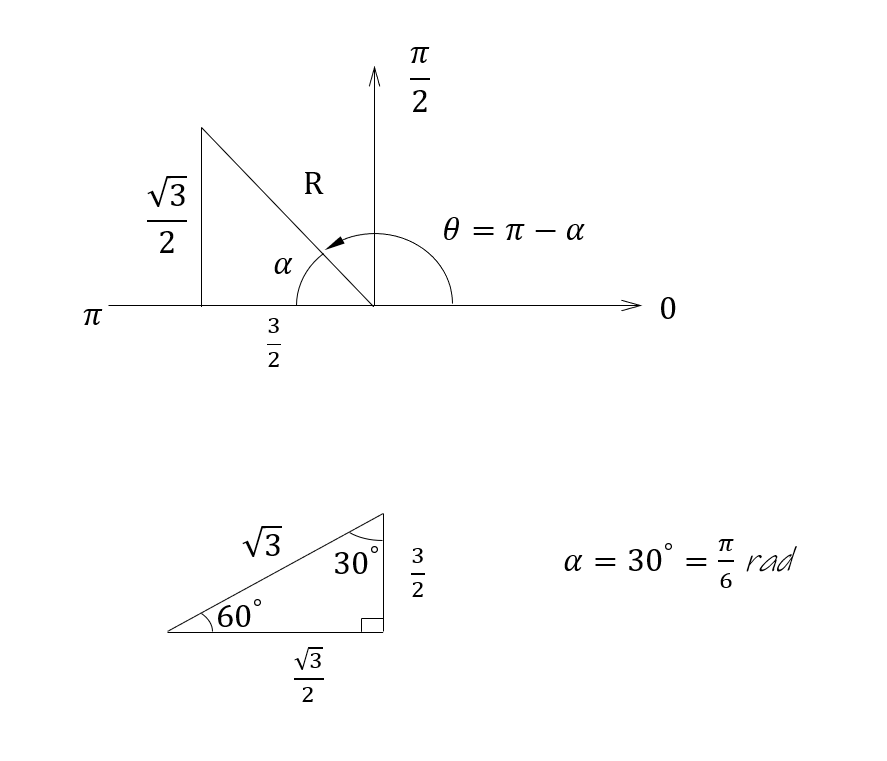
Complementary function $\Rightarrow x_{t}=(\sqrt{3})^{t}\left[A\cos\left(\frac{5\pi}{6}t\right)+B\sin\left(\frac{5\pi}{6}t\right)\right]$
More topics will be added here as this page grows.